Spreadsheets
Calculate with formulas that refer to cells, other sheets, named ranges and tables.
A formula in a spreadsheet starts with = and can use arithmetic, references and the built-in functions, from SUM and VLOOKUP to XLOOKUP, FILTER and LAMBDA. As you type, autocomplete shows each function's syntax and what it does, and a formula that cannot be calculated shows an error value that says why.
Get started free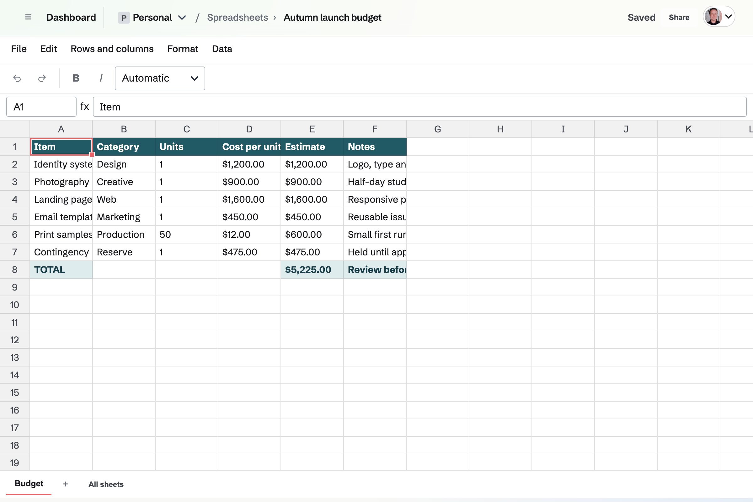
Cell references, other sheets and named ranges
The formula bar (fx) above the grid shows a cell's formula rather than its result. While you edit a formula, the cells it refers to are outlined on the sheet.
- Cells and ranges
- B2, B2:B11, and whole columns and rows such as A:A and 2:2. References can be relative, absolute or mixed ($A$1, A$1), and a copied or filled formula adjusts its relative references.
- Other sheets
- Sheet2!C7, or 'Annual Budget'!B7 for a sheet name with spaces. Renaming a sheet updates the formulas that use it.
- Named ranges
- Name a cell or range, such as TaxRate, and write =Revenue*TaxRate.
- Table columns
- A range converted to a table can be used by its column names, as in =SUM(Sales[Revenue]).
- Inserted and deleted rows
- Formulas keep pointing at the same cells when rows and columns are inserted or deleted.
Functions by group
Inside a function's parentheses, autocomplete shows its syntax with the argument you are typing in bold. These are the groups and most of their functions; the Help article lists every one.
- Math
- SUM and PRODUCT add and multiply; ROUND, ROUNDUP, ROUNDDOWN, CEILING and FLOOR round; MOD, POWER, SQRT, ABS, LOG, SIN, COS and TAN are included too.
- Statistics
- AVERAGE, MEDIAN, MODE, STDEV, MIN, MAX, LARGE, SMALL, RANK, PERCENTILE and FORECAST describe a set of numbers; COUNT, COUNTA and COUNTUNIQUE count values.
- Conditional sums and counts
- SUMIF, COUNTIF and AVERAGEIF take one condition, and SUMIFS, COUNTIFS, AVERAGEIFS, MAXIFS and MINIFS several. Criteria ignore case and accept * and ? as wildcards.
- Logic
- IF, IFS and SWITCH choose a result; AND, OR, NOT and XOR combine conditions; IFERROR and IFNA give a fallback for an error.
- Lookup and reference
- VLOOKUP, HLOOKUP, XLOOKUP and LOOKUP return a matching value, and MATCH and XMATCH its position; INDEX and CHOOSE pick a value by position. Text matches without regard to case.
- Text
- CONCAT, TEXTJOIN, LEFT, MID, LEN, UPPER, PROPER, TRIM, SUBSTITUTE, FIND, SEARCH and SPLIT work with text, and TEXT formats a number or date with a pattern such as #,##0.00.
- Date and time
- DATE, TODAY and NOW make dates; YEAR, MONTH, DAY and WEEKNUM read them; DATEDIF, EDATE, EOMONTH, WORKDAY and NETWORKDAYS count and move between them. Date text given to a function must be an ISO date such as 2026-08-23.
- Financial
- PMT, FV, PV, NPER, RATE, IPMT and PPMT work out loans and investments, NPV and IRR evaluate cash flows, and SLN, DB and DDB give one period's depreciation.
- Dynamic arrays
- FILTER, SORT, SORTBY, UNIQUE, SEQUENCE and TRANSPOSE return a range of results; VSTACK, HSTACK, TAKE and DROP reshape one.
- Value tests and random numbers
- ISBLANK, ISNUMBER, ISTEXT, ISERROR and ISFORMULA test a value; RAND and RANDBETWEEN return random numbers.
Results that fill several cells
Some formulas return more than one value: =SEQUENCE(10) fills ten rows, and =FILTER(A2:C100,C2:C100="Active") returns every matching row. The formula is in the first cell, and its results fill the cells beside and below it. Those cells cannot be edited or pasted over, and if something is in the way, the formula shows #SPILL! until it is moved or cleared.
Named functions, LET and LAMBDA
- Named functions
- Save a calculation you repeat with a name and parameters, such as PRICE_AFTER_DISCOUNT(PRICE, DISCOUNT) defined as =PRICE*(1-DISCOUNT). It can be used on any sheet, and autocomplete lists it with the built-in functions.
- LET
- Names values inside one formula, so each is written once: =LET(Net, B2-C2, Tax, Net*0.13, Net+Tax).
- LAMBDA
- Makes a calculation that MAP, REDUCE, SCAN, BYROW, BYCOL and MAKEARRAY apply to each value, row or column, as in =MAP(A2:A10,LAMBDA(V,V*2)).
Error values
A formula that cannot be calculated shows an error value in its cell. A formula with a typing mistake is still saved, and a message says what was expected and at which character.
- #ERROR!
- The formula cannot be read, or it is part of a circular reference.
- #REF!
- A cell, row, column or table it referred to was deleted.
- #NAME?
- It uses a named range or named function that does not exist.
- #VALUE!
- A function got the wrong number or kind of arguments.
- #DIV/0!
- It divides by zero, or averages a range with no numbers in it.
- #SPILL!
- Its results would cover cells that are not empty.
- #NUM!
- There is no number result, as in =SQRT(-1), or the results would fill more cells than one formula can.
- #N/A
- A lookup found no match.
Where formulas are calculated
Formulas are calculated in the spreadsheet on the website, and each result is saved with the spreadsheet. Export CSV writes the saved result for each formula cell. TODAY, NOW, RAND and RANDBETWEEN change when a change to the spreadsheet is saved, not while you type.
Write your first formula.
Create a Magpie account, open Spreadsheets and select New Spreadsheet, or import a CSV file to calculate with data you already have.